Visualising the Markov blanket

The Markov blanket of a variable \(X\) in a DAG is the set of nodes that, when conditioned on, renders \(X\) independent of every other variable — formally, the union of its parents, children, and the parents of its children (its spouses).

Extracting the Markov blanket

bnmetrics.markov_blanket(g, var) returns a sub-GraphLike restricted to \(\{X\} \cup \mathrm{MB}(X)\), preserving every endpoint mark incident to those nodes. bnmetrics.markov_blanket_indices returns the indices only.

import numpy as np
import bnmetrics

# 6-node DAG: A → C, B → C, C → D, C → E, D → E, E → F
endpoints = np.zeros((6, 6), dtype=np.int8)
for i, j in [(0, 2), (1, 2), (2, 3), (2, 4), (3, 4), (4, 5)]:
    endpoints[i, j] = 2
    endpoints[j, i] = 1
g = bnmetrics.to_graphlike(endpoints,
                     var_names=("A", "B", "C", "D", "E", "F"))

bnmetrics.markov_blanket_indices(g, "C")     # (0, 1, 2, 3, 4)
mb_c = bnmetrics.markov_blanket(g, "C")
mb_c.var_names                          # ('A', 'B', 'C', 'D', 'E')

Node F is excluded because it is a descendant of E but not a spouse of C. The MB of C is \(\{A, B\} \cup \{D, E\} \cup \{D\} = \{A, B, D, E\}\).

Plotting the Markov-blanket subgraph

bnmetrics.plot_graph accepts the MB subgraph directly. Highlighting the target node makes the blanket structure immediately legible:

bnmetrics.plot_graph(
    mb_c,
    title="MB(C)",
    highlight=["C"],
    direction="LR",
    save="mb_c.svg",
)

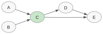
The highlight argument paints the listed nodes in a distinguishing colour (default pastel green); every other element follows the default style.

Comparing two graphs on the Markov blanket of a target

When two graphs are being compared and the analysis of interest is local to a particular variable, scope both graphs to the MB of that target before passing them to a metric or visualiser. The example below compares the true DAG above against a recovery that has dropped the \(D \to E\) edge:

endpoints_rec = endpoints.copy()
endpoints_rec[3, 4] = 0
endpoints_rec[4, 3] = 0
g_rec = bnmetrics.to_graphlike(endpoints_rec,
                         var_names=("A", "B", "C", "D", "E", "F"))

mb_true = bnmetrics.markov_blanket(g,     "C")
mb_rec  = bnmetrics.markov_blanket(g_rec, "C")

bnmetrics.shd(mb_true, mb_rec)              # 1 — the missing D → E edge
bnmetrics.plot_side_by_side(
    mb_true, mb_rec,
    name1="true_MB(C)", name2="recovered_MB(C)",
    direction="LR", save="mb_comparison.svg",
)

true MB(C)	recovered MB(C)

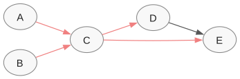
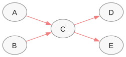
The MB-scoped SHD is identical to the global SHD here because the dropped edge falls inside \(\mathrm{MB}(C)\). In general the MB-scoped distance is a lower bound on the global distance, and the gap quantifies how much of the recovery error is local to the target.

Per-node Markov-blanket summary

bnmetrics.analyse_mb produces a multi-panel plotly figure summarising the per-node MB descriptive metrics (one panel per variable, faceted by metric). Each panel reports the descriptive metrics restricted to the corresponding MB subgraph:

fig = bnmetrics.analyse_mb(
    g,
    descriptive=["n_edges", "n_directed_arcs", "n_colliders"],
    cols=3,
)
fig.write_html("mb_summary.html")

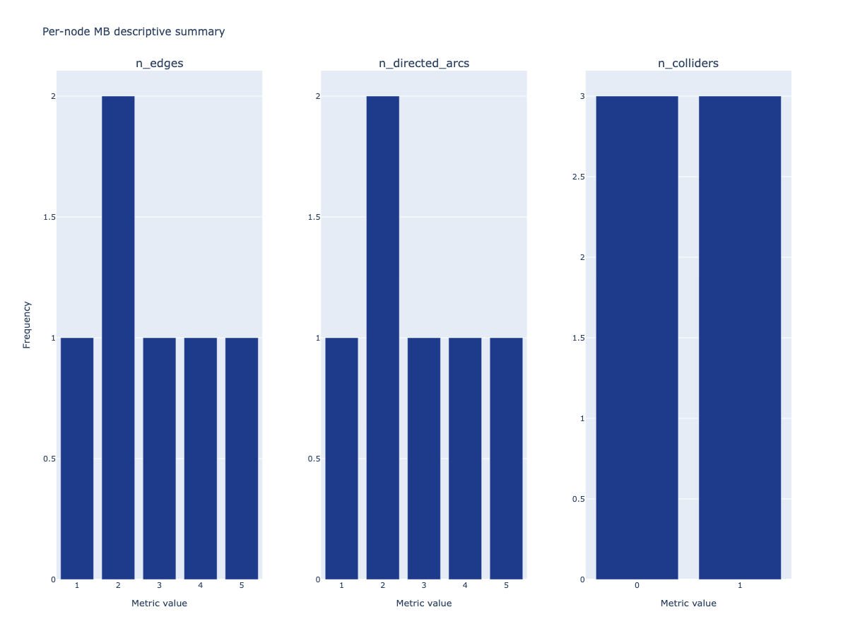
descriptive accepts either a list of metric names or the literal string "all". The figure is a standard plotly.graph_objs.Figure, so it can be saved with .write_html, .write_image (requires kaleido), or displayed directly in a notebook.